Turbulence Synthesis with Generative Adversarial Networks
This project involved exploring the use of GANs to generate so-called “fake” turbulence. I provided a brief overview of the dynamics of GANs in this post. The training data for this project were 2D horizontal slices of velocity fields in a direct numerical simulation (DNS) of turbulent channel flow. If you don’t know what a channel flow DNS is, it’s essentially a simulation where we are forcing fluid to flow through a rectangular box, and the DNS means that these simulations are very accurate and that we aren’t taking any shortcuts when it comes to solving the governing equations of fluid motion.
Not taking any shortcuts means these simulations are quite computationally heavy, and take a long time to simulate. The motivation around training a GAN to generate these flow instances is to have it act as an emulator - i.e the hope is that this GAN model can emulate fluid flow with the same precision as a DNS, in a fraction of the time.
Some of the limitations of this method is that as we increase the dimensionality of the data (i.e moving to 3D), the networks get prohibitively expensive, and it isn’t possible to train a network on my full simulation domain. It worked great for the small slices I was able to fit though - we’ll just have to wait for computing to catch up before moving to higher dimensional synthesis.
Some results of the project can be seen in the figures below:
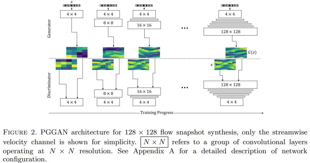
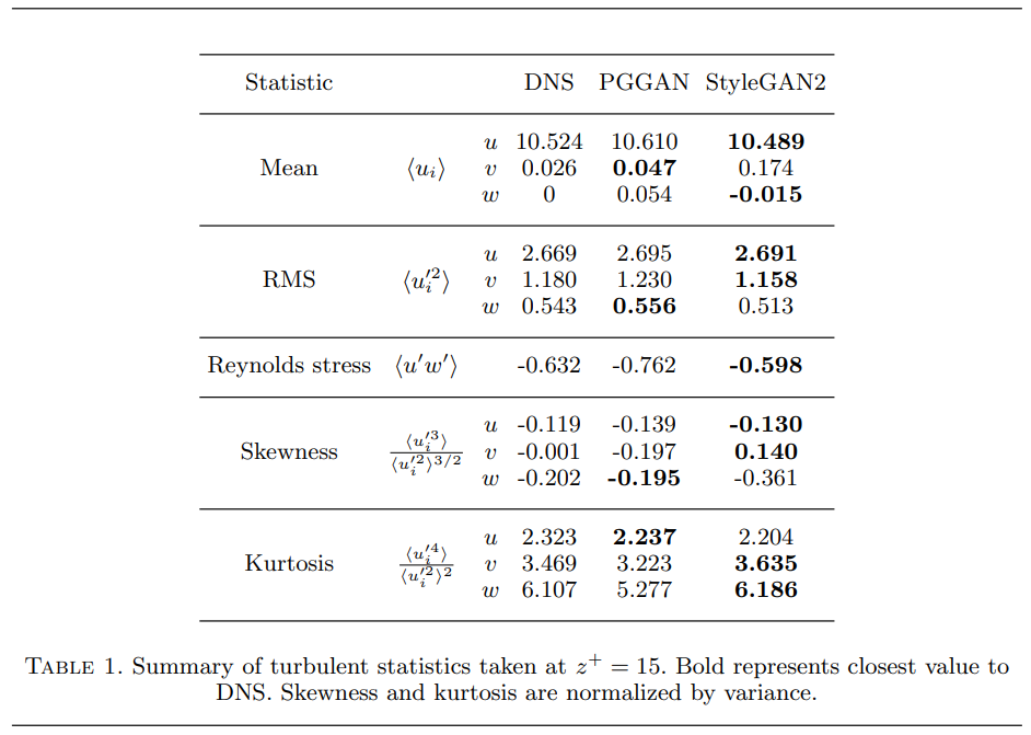
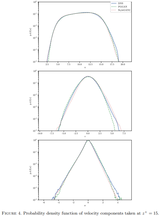
This table compares the statistics between the DNS velocity fields (true values) and samples generated from a PGGAN (see Figure 2 above for archichture overview) and StyleGAN2 architecture. These values essentially describe the shapes seen in the probability distribution functions seen in Figure 4 below. Here u, v, and w are the streamwise, spanwise and wall-normal velocities, respectively.
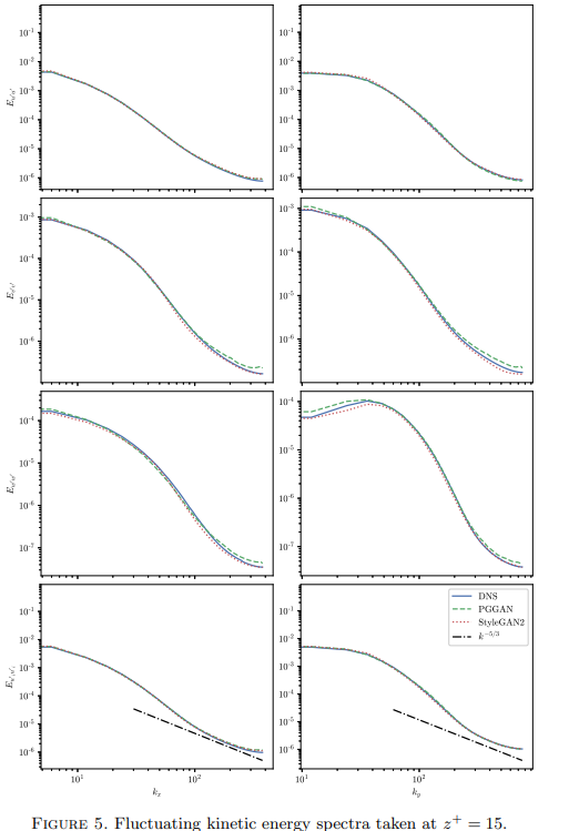
Energy spectra comparisons are used to see whether the generated fields correctly transfer energy between different length scales. In turbulence, the way energy is distributed is from the large scales (think large sweeps of air) down to smaller and smaller scales (little sweeps of air) until eventually this kinetic energy fizzles out into heat (this happens at what we call the dissipative scales).
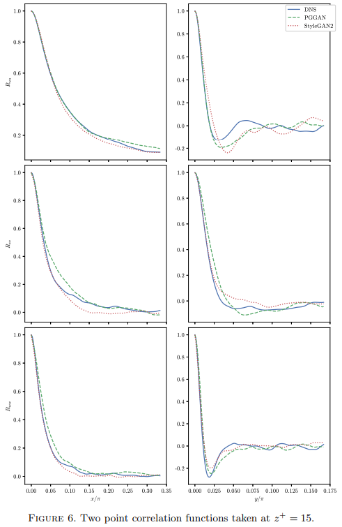
Two point correlation comparisons are used to see whether the spatial behaviour of velocity values are correctly reproduced. A correlation of zero here means that the two values are uncorrelated (i.e just noise relative to each other). The top right plot here represents the two point correlation of streamwise velocities in the spanwise direction. Normally in channel flow near the wall, you end up getting these alternating high and low speed streaks arranged along the spanwise direction. This is why the correlation function dips below zero, spring up a little above zero, and eventually zeros out. You can see that the generative models struggle to correctly reproduce this behaviour in their samples. This could be corrected via a statistical regularizer in the generator’s loss function.
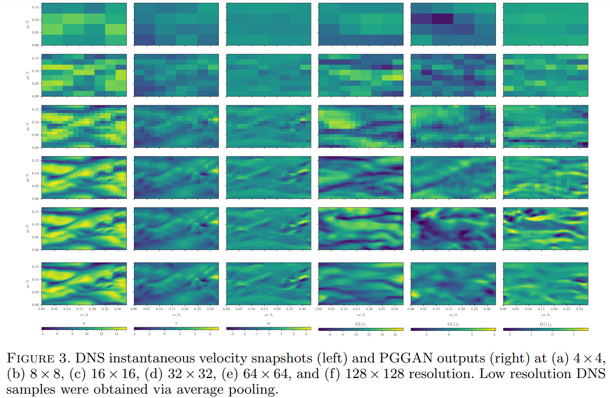
Here are some qualitative results obtained throughout the PGGAN training process. The three plots on the right hand side are synthetic fluid fields generated by the PGGAN at different scales. The StyleGAN2 results were comparitive to these, so they are not shown.
The interesting thing about StyleGAN2 is that you can apply the truncation trick. This involves truncating the latent space that we are sampling from, and what we can end up doing is selectively choose to generate images from the edge of our distribution. This translates to less frequent samples - or more unique samples. You can imagine it like this, say I do this for a distribution for human faces. By using the truncation trick, I can generate faces with less frequent, more unique features such as a man with a moustache and glasses. Likewise for fluid dynamics, this translates to flow instances with localized high/low magnitude velocity values. In other words, it offers the ability to generate the otherwise infrequent intermittent events found in turbulence.

